In our first post, we talked about the basics of artificial neurons and the inspiration from their biological counterparts. In this post, we will understand the inner workings and see how a neural network actually works, without the technical math details (to make it simpler to understand).
How Does a Neural Network Work?
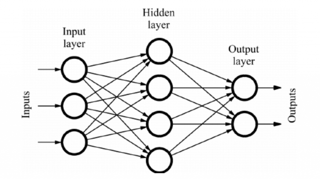
A typical neural network consists of an input layer, hidden layers, and an output layer. Each layer has a specific number of nodes (a node is an artificial neuron). The input layer is where the data enters the neural network. The hidden layers are where the neural network processes the data. The output layer is where the neural network outputs the results of the processing.
The input layer contains neurons that receive the input data. The hidden layers contain neurons that process the data. The output layer contains neurons that output the results of the processing.
The goal of training a neural network is to adjust the weights and biases of the neurons in such a way that the output of the neural network is close to the desired output for a given input. This process is known as training the neural network.
FeedForward and Backpropagation
Once we have initialized a neural network, we need to train it. Training means setting the right values of weights and biases so that the neural network can output the correct values on actual data set.
When an input value is “fed” to the neural network, it is fed through the input nodes and propagated (“fed forward”) through the hidden layers until it reaches the output node. At each node, the input value is multiplied by its associated weight, summed up, and passed through an activation function. This process continues until the input value have been passed through all the hidden layers and reaches the output node.
The output node then calculates an error value based on how close its output value is to the desired output value. This error value is then propagated back through the hidden layers until it reaches the input node. At each node, the error value is multiplied by a weighting factor. This process continues until the error value has been multiplied by every weighting factor and reaches the input node.
The last step in backpropagation is to update the weights & biases of all of the connections between nodes based on these calculations. We employe “gradient descent” approach to adjust weights and biases during backpropagation. This process is repeated for each input/output pair until all of them have been used, and all of the weights have been updated.
Gradient Descent
The idea behind backpropagation is that we can use gradient descent to adjust the weights of the connections between nodes so that the error between the predicted output and the actual output is minimized.
To do this, we need to calculate the partial derivative of the error with respect to each weight in the network. This can be done using the chain rule. Once we have all of the partial derivatives, we can update the weights accordingly and repeat the process until the error is sufficiently small. To read more about the mathematical details behind gradient descent, please watch this video and refer this blog post.
So to summarize, a neural network is initialised by setting random values for its weights and biases. Then the neural network is trained on a large dataset so that we can use backpropagation and gradient descent to adjust the weights and biases so that the error is minimum. Once the error between input and output values are within acceptable levels, we can say that the network is now trained and ready to be used for real-world datasets.
Conclusion
In this post, we talked about the inner workings of a neural network from a very high level perspective. Stay tuned for our next post where we will be discussing different types of neural networks and their practical uses.